iGrafx Client Tutorial

About this Tutorial

These topics in this page help you get started with basic diagramming, modeling, and analysis tasks if you are new to these iGrafx Client tools:

• iGrafx FlowCharter
• iGrafx Process
• iGrafx Process for Six Sigma

Some topics build on the first topic, Create a Process Map, so be sure you are familiar with the concepts in that topic before you begin another tutorial. If you cannot finish all the tutorials in one session, save your work. From the File menu, choose Save As and choose a different file name. 

See the iGrafx client Help menu for reference and other information. From the Help menu, choose iGrafx Help. 

In addition, click the link below for a 13 minute video demonstration of process mapping with the iGrafx Client.

Process Mapping with the Client.mp4

Create a Process Map

In the iGrafx QuickStart dialog box, click the Process template category, and choose Cross- Functional Process. If you have already closed the QuickStart dialog box, on the File menu, select New, then, in the resulting New dialog box, click on the Process template category, then the Cross-Functional Process template, and click OK. 

Topic Tasks

Apply a Color Theme to the Diagram
Place Text in Shapes
Connect Shapes
Add Swimlanes
Rename Swimlanes and Move Shapes between Swimlanes
Create Cross-Swimlane Activities
Customize the Shapes on the Toolbox Toolbar
Specify Automatic Numbering
Create Hierarchy (Links to Diagrams in the Same File)
Create Links to External Files
Add Notes
View Off-Page Connectors
Scale a Page for Print Output
Published Output

Place Shapes (Activities)

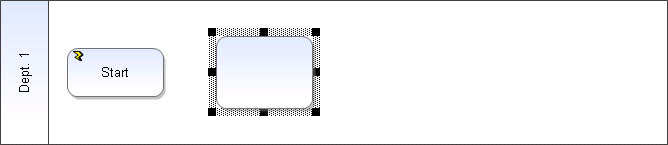
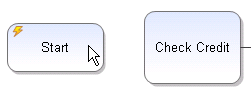
The Cross-Functional Process template includes a Start shape and a Swimlane® (Dept. 1) in the new diagram. 

Place a rectangle (activity) in the diagram:

1. Click the rounded rectangle (Activity) shape on the Toolbox toolbar.
2. Move the cursor into the diagram.
3.  The cursor changes to the placement cursor:
    

   

4. Press and hold the left mouse button while you move (a.k.a. click and drag) the mouse to place the shape to the right of the Start shape in the diagram, then release the mouse button when the shape is where you want it.

 

The iGrafx auto-sensing feature changes the cursor to the selector and line drawing 

 tool and remembers the shape you were placing so that you can quickly move shapes, draw lines, and select objects, then return to placement mode when you click in empty space. 

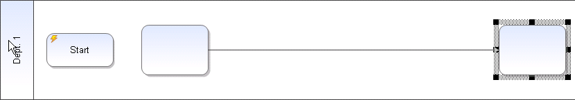
1. Click in empty space, then place the cursor over the existing rectangle shape. The cursor changes to the place and connect cursor: 
   

   

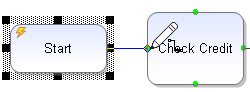
2. Click and drag (click-hold-drag the mouse) from inside the first shape you placed to the right of the swimlane boundary, and release the mouse button.
3. Leave the shape you just placed selected.
   
   

 

Apply a Color Theme to the Diagram

By default, swimlane name areas, shapes, graphics, and phase name areas apply a color fill from the theme; the swimlane process areas are not filled.

1. From the View menu, choose Themes.
2. In the Themes window, click a color theme.

To change the default settings of how themes are applied in your diagram:

1. In the Themes pane, click Setup Diagram Colors.
2. In the Setup Diagram Colors dialog box, select a check box and change the theme color in the drop-down list to apply color settings to diagram objects. If you want to apply colors to one object at a time, you can select the object and from the Format menu, choose Fill.

Objects that have been set to a theme color will be updated with a new color if a different theme is selected. Objects that have been set to Automatic, None, Standard Colors or Custom Colors will retain these settings regardless of the theme. 

Move and Grow Shapes

Adjust the placement of shapes by moving them:

1. Click the right-most rectangle shape if it is not already selected.
2. Place the arrow cursor directly on one of the light gray stippled border areas (but not a corner) of the selected outline of the shape. The cursor changes to indicate it can be used to move a symbol:
   

   

3. Click and drag the shape to try moving it around, but return it to its position on the second page (to the right of the vertical dashed line).

Grow a shape:

1. Click the shape if it is not already selected. If necessary, press the Esc key to temporarily leave another mode.
2. Place the cursor on a dark square at the corner of the selected outline. The cursor changes to a double-headed arrow.
3. Click and drag the grow handle to a new location. A shape outline indicates how the shape grows.

Place Decision Shapes

Place a diamond (intelligent decision) shape in the diagram:

1. Click the diamond shape in the Toolbox toolbar.
2. Move the cursor into the diagram.
   
   The cursor changes to the placement cursor. 
   
   
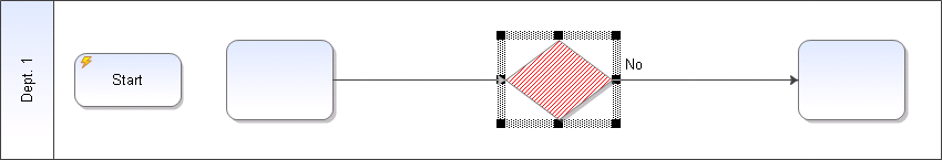
3. Click and drag the outline of the decision shape to place it on the connector line between the two Activity (rectangle) shapes.

Connector lines are automatically created with decision case labels on decision shapes. By default, the first line drawn from a diamond is labeled No and the second is Yes. You can define your own label text. 

 

If your lines aren't straight, try moving a shape. You may also select multiple shapes (use the Ctrl or Control key and click) and on the Arrange menu, choose Align. 

Place Text in Shapes

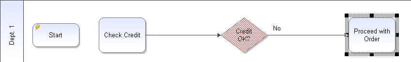
Label the shapes:

1. For each shape, click to select the shape and type text as shown below.
2. Click the selector tool on the Toolbox toolbar or press the Esc key to leave text entry mode when you are finished.
   
   

 

Connect Shapes

Within a process diagram, shapes represent steps of the process. Connected shapes can show the flow of the process. 

Connect the remaining shapes:

1. Click the selector tool in the Toolbox toolbar if it is not currently active. If necessary, press the Esc key to temporarily leave another mode.
2. Move the cursor inside the Start shape boundary, near the right side.
   
   

   

3. Click and hold the mouse button and drag to the inside of the left side of the Check Credit shape.
   
   

   

    
   
   
4. Then, release to draw the connector line. The click-hold-release action is also known as click and drag.

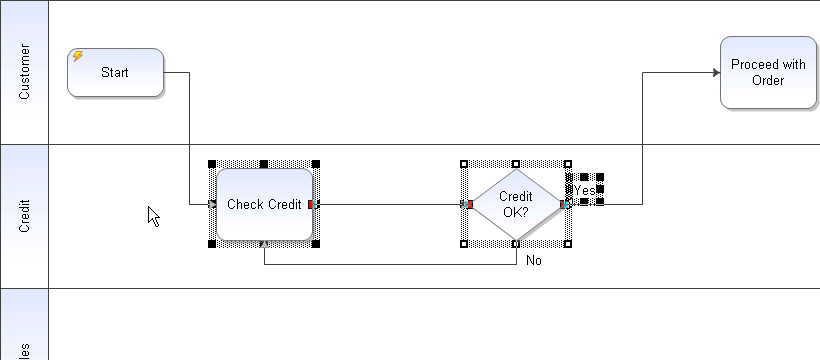
Connect the bottom of the decision back to the Check Credit rectangle:

1. Move the cursor inside the diamond shape boundary.
2. Click-hold-release (click and drag) slightly inside the bottom of the Check Credit shape.
   
   

   

    

Change Output Labels:

1. Right-click over the No text label next to the decision.
2. In the resulting context menu, choose "Yes."
   
   iGrafx automatically changes the other label from Yes to No when you change this label. 

Add Swimlanes

Swimlanes in iGrafx can represent many things, like resource specialization and cost centers. 

Add swimlanes to the diagram:

1. Click the selector tool, then click empty space in the diagram to clear object selection.
2.  Click the Swimlanes tool

   

    on the Toolbox toolbar and choose Insert Swimlane.
3. Type the swimlane name "Credit" and leave the location as Top Level.
4. Click the Apply button. The Credit swimlane is added below Dept. 1.
5. Type the swimlane name "Sales" and click OK.

You now have three swimlanes: Dept. 1, Credit, and Sales. 

Rename Swimlanes and Move Shapes between Swimlanes

Rename swimlanes:

1. Ensure the selector tool is active.
2. Click to select the swimlane name area labeled Dept. 1 and type "Customer."
3. Click in empty space in the diagram to clear object selection.

Lasso select shapes:

1. Ensure the selector tool is active.
2. Place the cursor above and to the left of the Check Credit shape. Do not click on the shape.
3. Press-hold-release (click and drag) to below and right of the Credit OK? shape so that the blue selection box is drawn completely around the objects.
   
   

   

    

Move the selected shapes into the Credit swimlane:

1. Place the cursor over the light gray border of one of the shapes.
2. Move (drag) the selected shapes into the Credit swimlane:
   
   

   

    
   
   The swimlane automatically resizes to accommodate shapes. 

Create Cross-Swimlane Activities

Normally, swimlanes expand to accommodate shapes, but you can model an activity that spans across (involves) multiple swimlanes. 

Create a cross-swimlane activity:

1. Select the Proceed with Order shape.
2. Press and hold the Ctrl (Control) key and place the cursor over a dark square on the bottom of the shape.
   
   

   

    The cursor changes to the cross-swimlane cursor.
   
   
3. Click and drag to expand the shape across all three swimlanes while holding the Ctrl key.
4. Release the mouse button before you let go of the Ctrl key. 

Exclude a swimlane from a cross-swimlane activity:

The Credit swimlane is not involved in the activity.

1. Double-click the cross-swimlane shape, or right-click and choose Properties.
2. In the resulting Properties dialog box, click Task, under Modeling.
3. On the Task page's Step tab, click the Exclude Swimlane... button.
4. In the Swimlanes list, click Credit, then click the Yes button to exclude the swimlane.
5. Click OK to close the Exclude Swimlanes dialog box, then click Apply in the Step tab of the Properties dialog box.
   
   The excluded swimlane (Credit) displays a dashed outline. 

Customize the Shapes on the Toolbox Toolbar

By default, three shapes are available on the Toolbox toolbar. You can add or delete shapes in the toolbar at any time.

1. Click the right arrow underneath the decision (diamond) shape in the Toolbox toolbar.
2. Click Shape Library.
3. Click the Add Shapes button in the Shape Library dialog box.
   
   The shape palettes appear on the right-hand side of the dialog box.
   
   
4. Click a shape, and then click the Add button to add it to the Shape Library.
   
   The check mark next to the shape indicates it is visible on the Toolbox toolbar.
   
   
5. Click the Close button.

Specify Automatic Numbering

iGrafx numbers shapes in the order they were placed in the diagram. You can use the Auto Renumber and Manual Renumber tools to number the shapes in any order. iGrafx does not create duplicate numbers. 

Display shape numbers:

Click the Shape Numbering tool 

 in the Toolbox toolbar and choose Show All Shape Numbers. To renumber shapes, click the Shape Numbering tool, choose Auto Renumber, choose a Renumber Style (e.g. By Flow through Diagram), and click OK. 

Create Hierarchy (Links to Diagrams in the Same File)

You can easily capture top-down processes and drill down into successive levels of detail in connected diagrams. 

Create a subprocess for the Check Credit activity shape:

1. Right-click the Check Credit shape and choose Add Subprocess.
   
   Alternatively, use the Properties dialog box. To do so, do the following:
   • Double-click the shape (or right-click on it and choose Properties).
   • In the Properties dialog box, click the Guide page under the Shape category.
   • From the Activity Type drop-down list, choose Subprocess.
   • Click the New button.
   • Follow the steps below.
     
     
2. Type "Check Credit" in the New Component dialog box.
3. Click OK on all open dialog boxes. The Check Credit subprocess appears.
   
   Optional: Create the Subprocess
   
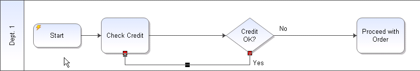
   For more practice, draw the diagram below using the steps in prior sections (you may delete swimlanes you do not need by clicking on them to select them and then pressing the Delete key). 
   
   

   

    
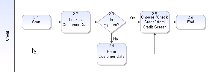
   This process is shown in landscape page layout, which is the default. If you want to change this, on the File menu, choose Page Setup and click the Page tab to choose another layout.
   
   
4. Close the Check Credit Subprocess diagram window.

You may have multiple diagrams in a single file. You can use the Document Components window (on the View menu, point to More Windows and choose Document Components) to view all of the components of the file, or even the hierarchical structure of the diagrams. 

Create Links to External Files

Link to a file created in another application:

1. Select the Start shape on your Process1 diagram.
2. From the Insert menu, choose Link.
3. In the Add Link dialog box Link to section, click File or Web Page in the "Link to" section on the left.
4. Click the web page icon. This may display your web browser so you can find a web page. Close the browser when you have displayed the page you want, and the path (URL) to the page will be entered for you. If a path is not entered, type or paste one in. For example, you could type http://www.igrafx.com/
5. Click in the Key Modifiers box and press the Ctrl key, the Shift key, the Alt key, or a combination of those keys.
   
   This designates a special keystroke that you will use with double-click to view the linked file. 
   
   
6. To add a description, click the Custom option, then type a description in the Description box.
7. Click OK.

The shape now has a link, indicated by an icon that represents the default browser on your machine. If you create multiple links, a default link icon is used. 

Activate (follow) the link:

Right-click on the shape and choose the link you created, or press and hold the key you designated as a key modifier (e.g. the Ctrl key) and double-click the shape to view the linked web page. 

Add Notes

Make a note of what the linked data is and why it's referenced:

1. Select the Start shape, if necessary.
2. From the View menu, choose Note, or press the F6 key.
3. In the note window, type "Work Instructions and form for this step."
4. Close the Note window.
   
   A default icon

   

    on the shape indicates a note. 

Place your cursor over the shape to see the note text in a ToolTip. (To activate ToolTips display on notes, from the View menu, choose Note Tooltips.) 

View Off-Page Connectors

Add off-page connectors for a process that spans multiple pages:

1. From the Format menu, choose Diagram.
2. Click the Off-Page Connectors tab.
3. Select the Automatic Connectors check box and the Include Page Numbers check box.
4. Choose the shape you want for your off-page connector (e.g. Directional).
5. Click OK.

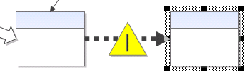
The off-page connectors now display at every page boundary. The following picture shows a generic example of off-page connectors: 

 
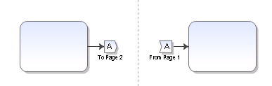
Page boundaries are indicated by the dashed gray page break lines (not to be confused with the dashed phase lines). If necessary, zoom out far enough to see the page boundaries. 

Scale a Page for Print Output

Fit the diagram to a certain number of pages of a specific size:

1. From the File menu, choose Page Setup.
2. Select the Page tab, if it is not already selected.
3. In the Scaling section of the dialog box, click the Fit to option and enter 1 page(s) wide by 1 tall, then click OK.

The page connectors automatically disappear because the complete diagram now prints on a single page. 

Published Output

You can easily publish diagrams to a web format that any internet browser can display, or to Adobe® Acrobat® PDF, Microsoft® Word or PowerPoint® format for viewing without iGrafx. You may also install the iGrafx Viewer® to view iGrafx Client documents.

If you have the iGrafx Platform, repository items may be viewed via browser. 

Publish as PDF:

1. From the File menu, point to Publish As and choose PDF Document.
2. Change the publishing options if desired (click the Help button if you want help with the features), and click OK.
3. Click Yes when iGrafx prompts you to open the new document.
   
   Your PDF reader (such as Adobe® Acrobat Reader®) opens and displays one page with a picture of the process and any header and footer information specified in the Page Setup dialog box. 

Create Lean Value Stream Map Diagrams

Lean value stream map (VSM) diagrams and data employ some esoteric terminology, and this tutorial assumes that you are familiar with it. It may be helpful for you to review the iGrafx Help system documentation on Lean terms and calculated data. 

In this topic, first you set the overall VSM properties that control options for the map, then you draw the diagram, enter and customize data, and export data.

Topic Tasks

Set Lean VSM Properties
Create a Lean VSM
Create Hierarchy in a Lean Value Stream Map
Customize Data Entry
Export VSM Data

Set Lean VSM Properties

The Lean VSM properties control analysis and display options for the VSM.

The Timeline tab of the Value Stream Map Properties dialog box controls display of calculated values and other analysis information. 

Start a new document and set up Lean VSM properties:

1. From the File menu, select New. In the resulting New dialog box, choose Value Stream Mapping under Template Categories, and then select the Lean Value Stream Map template and click OK. A a new Lean VSM diagram opens, using the template (starting point) built into iGrafx.
2. From the Lean menu, choose Value Stream Map Properties. The Diagram Properties dialog box appears, showing the Setup tab for the first Lean timeline.
3. In the Setup tab, select the Use Custom check box for Available Work Time, and change or choose settings to match those shown here:
   
   

   

    
   
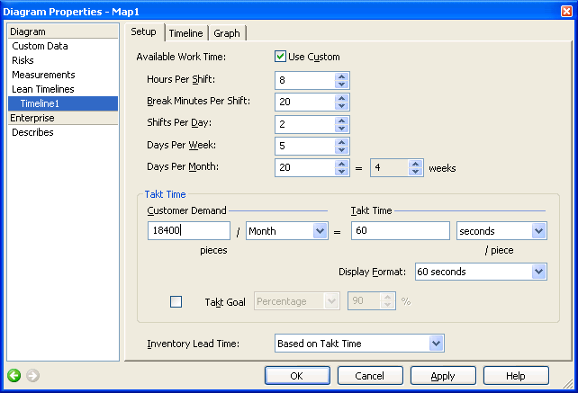
   When you set Customer Demand to 18,400 pieces with the given Available Work Time settings, iGrafx calculates a Takt Time of 60 seconds per piece. The Takt Time is a calculation of how often you should produce your product or service to synchronize the pace of production with customer demand. Note that you can set the units for Takt Time as well. 
   
   
4. Click the Timeline tab in the Timeline1 section of the Diagram Properties dialog box. Properties shown here display on the Timeline.
   
   

   

    
   
   
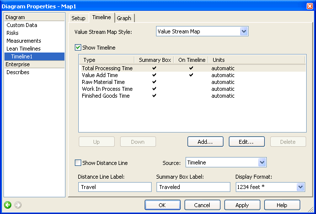
5. Click the Graph tab and select the check boxes shown here to display on the Work Balancing Graph.
   
   

   

    
   
   
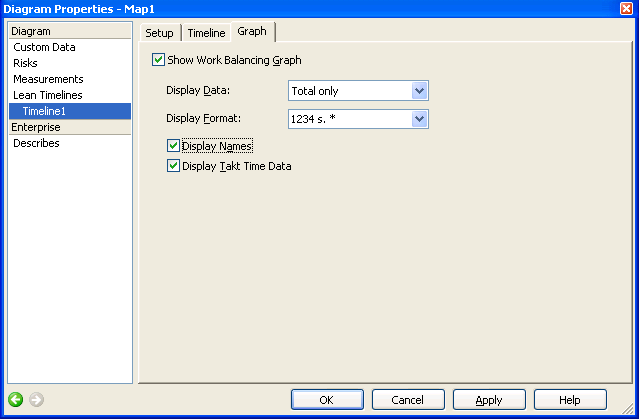
6. Click OK to save your choices and close the dialog box.

Create a Lean VSM 

Place shapes and lines, and label shapes:

1. Open the VSM Standard shape palette in the Shape Palettes window. If the Shape Palettes window is not visible, press the F9 key, or, from the View menu, choose Shape Palettes, then in the resulting Choose Shape Palette dialog box, expand the Lean branch, click VSM Standard, and then click the OK button. The VSM Standard shape palette tab is opened in the Shape Palette window.
2. Click the Truck 

   

    graphic in the VSM Standard shape palette.
3. Move your cursor into the diagram space so it changes to the placement cursor.
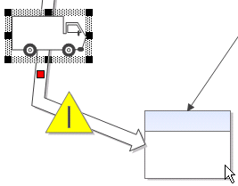
4. Click and drag the outline of the shape, placing it on the line at the left of the diagram, between the Supplier factory shape and the inventory triangle as shown after the next step.
5. Click and drag the attachment point (the red dot in the middle of the truck) onto the line. This section of your diagram may now look like this:
   
   

   

    
   
   
6. Click the Process 

   

    shape in the Toolbox toolbar.
7. Move your cursor over the first Process step, and the cursor changes to the place-and- connect cursor.
8. Click and drag from the first Process step to the right of where you placed the truck icon. This section of your diagram may now look like this:
   
   

   

    
   The default push line automatically places an inventory shape on the line, since current- state processes usually push product independently of demand, and thereby create inventory. 
   
   
9. Click the first Process step (shape) to select it, then click it again to place the text cursor on it.
10. Type "Stamping" to name the Process step.
11. Click the next step twice and name it Weld1.
12. Press the Esc key to exit text mode, or simply click in a white-space area where there are no objects.

Enter basic process data:

1. Right-click the Stamping shape and select Properties (or double-click it) to display its properties.
2. On the Lean page of the resulting Shape Properties dialog box, set the values and units of time as shown here. (You may use the Tab key to move to a new field.)
   
   

   

    
   
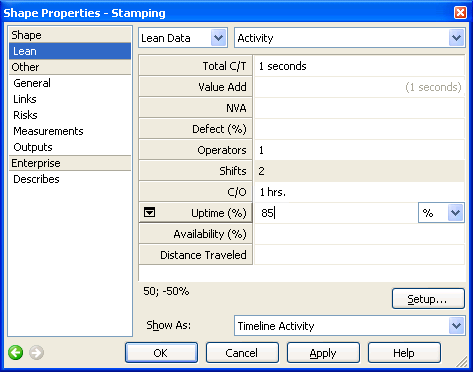
   Information such as the number of Shifts is automatically filled in (inherited) from the Diagram Properties dialog box settings. If you want to customize the data names to match your specific needs, click the Setup button. 
   
   
3. Click the Weld 1 step and set the value of Total C/T to 39 seconds, 1 Operators, C/O of 10 minutes, and Uptime (%) of 100.
4. Click the inventory triangle to the left of the Stamping step, and for Inventory Time type 5 and choose days for the units.
5. Click on the inventory triangle between Stamping and Weld 1, and for Pieces enter 7000.
6. Click OK to save your changes and close the dialog box. This section of your diagram may now look like this:

 
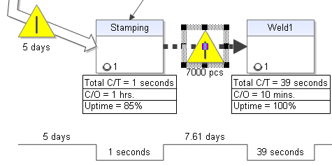
The timeline automatically calculates and displays the lead time (value-added and non-value- added time) data on the timeline. 
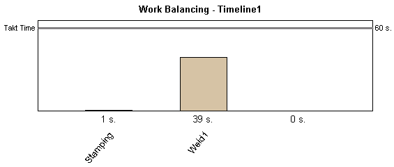
The Work Balancing graph also updates to show the Total C/T of each step and its relationship to Takt Time: 

 

Create Hierarchy in a Lean Value Stream Map

A typical value stream map (VSM) begins with the overall facility, but can have sub-maps that drill down into specific steps in the VSM, which are themselves VSMs for particular areas. There is a parent/child hierarchy between VSM for the whole facility and the VSMs for specific areas, allowing you to roll up data to the parent VSM.

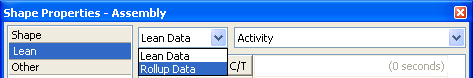
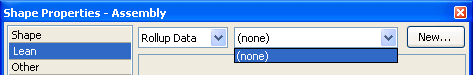
1. Add a step called Assembly and double-click it. The Shape Properties dialog box appears.
2. Click the data mode drop-down menu at the top left, that currently says Lean Data, and change it from Lean Data to Rollup Data.
   
   

   

    
   
   
3. You would have the option to choose other VSMs if they existed already in the document, or you can create a new VSM.
   
   

   

    
   
   
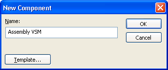
4. Click the New button to create a new child VSM.
5. In the resulting New Component dialog box, type "Assembly VSM" as the new VSM name.
   
   

   

    
   
   
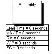
6. Click OK. The timeline data appears, showing default values from the Properties dialog box.
7. Click OK to close the Properties dialog box. A drop shadow appears on the process step to indicate a hierarchical link to another VSM.

 

Customize Data Entry

You can customize the data entry fields to meet your needs. For example, you want to track pieces of inventory for left-hand (L) and right-hand (R) configurations of steering columns, you can do that as described below. 

Set up and display custom data fields:

1. Double-click the inventory triangle between Stamping and Weld 1 to display its Properties.
2. On the Lean Data page, click the Setup button in the lower-right corner of the dialog.
3. In the Setup Custom Data dialog box, click to select Pieces in the Custom Data list.
4. Click the Rename button and type "Left" for the name.
5. In the Display As field, select the text that says pcs and change it to L.
6. Click the New button and type "Right" for the new custom data name.
7. In the Lean Types drop-down list, choose Inventory Amount.
8. Change the Display As field to display %v R.
9. Click the Up button (in the lower-left corner of the dialog box) enough times to move the new data field named Right to below the Left field.
10. Click OK to save your changes and close the Setup Custom Data dialog box.
11. In the Shape Properties dialog box, give the Left field a value of 4600 and the Right field a value of 2400, then click OK. The inventory triangle should now look like this:

 

Export VSM Data

You can export the data you've entered into your value stream map to Microsoft® Excel®. 

Export all your VSM data to Excel:

We will now export all of the data in our VSM to Excel (this requires Microsoft Excel to be installed on your computer):

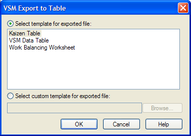
1. From the Lean menu, choose Export VSM Table to Excel. The VSM Export to Table dialog box appears:
   
   

   

    
   
   
2. Choose the VSM Data Table template and click OK.
   
   Excel starts (if it was not already started), and displays a worksheet with the information you asked iGrafx to export. You may now use Excel functionality to perform calculations or to do other analysis. 

Process Behavior Models

During process simulation, iGrafx gathers statistics on resource utilization, cycle (lead) time, costs, capacity, and other pre-defined and customizable statistics. 

A process model consists of activities (shapes), resources, and rules that govern process behavior. Transactions arrive at the input of an activity from a generator, or can be generated within an activity, and resources assigned to the activity may perform a task on each transaction. When the task is completed, the transaction is output (passed on to) the next activity through a connector line.

This tutorial provides a review of the behavioral modeling features of iGrafx FlowCharter. See What-If Analysis and Simulation for the what-if capabilities of simulation in iGrafx® clients that have simulation capability (e.g. iGrafx Process for Six Sigma). 

Topic Tasks

Specify Activity Task Duration
Specify Activity Resources
Specify Organization Resources
Choose Generators
Specify Run Setup

Specify Activity Task Duration

Set a distributed duration:

1. Open the ACME_Order (ACME_Order.igx) sample file (available at http://www.igrafx.com/support/documentation/sample-files), if not already open.
2. Right-click the shape (activity) labeled Check Credit, and choose Properties.
3. Click the Guide page in the Shape category (if not already selected); this is also known as the Process Guide or the Shape Guide.

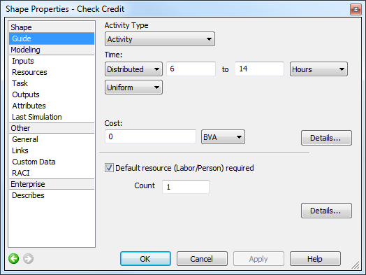
On this page, you enter information about the time duration of the activity, resource usage, additional cost per transaction, and value classification. For example, the duration can be based on an average, and identical for every transaction processed.

Set a Constant duration:

1. From the Time drop-down list, choose Constant (instead of Distributed).
2. Type the number "10" in the duration field, to the right of the Time drop-down list.
   
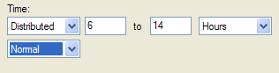
   Maybe the duration time is best defined as distributed between two values. For example, the duration of this activity for each transaction could vary randomly between 6 and 14 hours, with a normal or bell-curve distribution. In this case:

1. From the Time drop-down list, choose Distributed.
   
   iGrafx remembers that this step had 6 in the first box (minimum), and 14 in the second box (maximum). 
   
   
2. Choose Normal (in the drop-down list that currently says Uniform, under the drop-down that says Distributed).

 

The duration can be defined as an expression where the time span is defined by one of many built-in functions. 

Define powerful durations using statistical functions:

1. From the Time drop-down list, choose Expression.
2. Click the Expression Builder button

   

    in the text box to the right of the Time drop-down list.
3. Click the f(x) button 

   

    in the Expression Builder dialog box.
4. Scroll the list of possible functions that can be used in the Paste Function dialog.
5. Notice that the Normal distribution (NormDist) is one of many functions available.
6. Click Cancel to exit the Paste Function dialog box w/out saving changes.
7. Click Cancel to exit the Expression Builder.

Reset the time duration back to Distributed:

1. From the Time drop-down list, choose Distributed. It displays the proper time distribution of 6 to 14 Hours and remembers our last choice of Normal vs. Uniform.
2. Leave the Properties dialog box open.

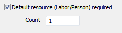
Specify Activity Resources

For each activity, you can specify the resources the task requires to process a transaction. By default, one resource is assigned for an activity, but you can change the number of resources in the Default resource (Labor/Person) required section of the Process Guide. Note that "Person" is the name of the default resource for an organization or department represented by a swimlane.

 

1. Click Cancel, to cancel your changes (we did not end up making any changes) and close the Properties dialog box.

Specify Organization Resources

You can view the resources available to the organizations represented by swimlanes within the process. As mentioned above, the shapes representing activities acquire these available resources.

1. From the Model menu, choose Resources or click the Resources button 

   

    on the Modeling toolbar.
2. Click the + icon next to Person and then click "C & I" which represents a set of workers with common attributes.
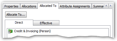
3. If not already visible, choose the Properties tab.
   
   The cost and count data properties are displayed for the Persons allocated to the "Credit & Invoicing" organization (which is represented by the "Credit & Invoicing" swimlane in the diagram).
   
   

   

   
   
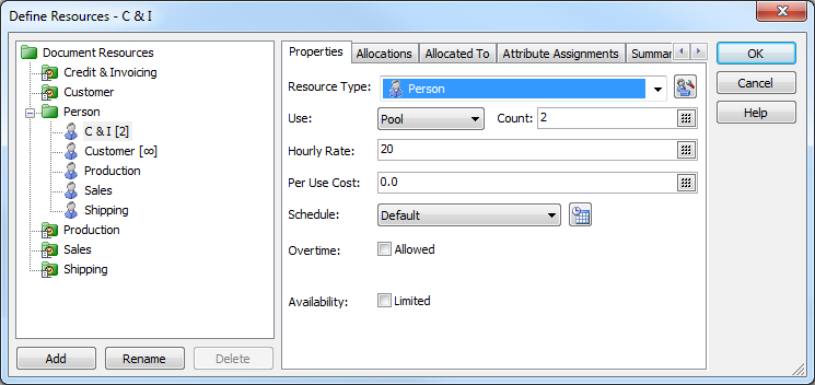
   When drawing a diagram, any swimlane containing activities that acquire workers will automatically get an organization created and an initial person resource allocated to the new organization. 
   
   
4. Click the Allocated To tab and within that tab choose the Direct tab
   
   This displays that the "C & I" persons are allocated to the "Credit & Invoicing" organization which is represented by the "Credit & Invoicing" swimlane on the diagram:
   
   

   

   
   
   
5. The allocation of person resources to organizations is necessary if you later wish to perform analysis and simulation.
6. Click the Cancel button, since we are not changing resource data at this time.

In the What-If Analysis and Simulation section of this tutorial, you can change the resource levels and see the impact on resource utilization. You can also use this dialog box to apply costs and schedules to your resources.

Choose Generators

During a simulation, a generator creates and sends transactions into the process. In this example, the transactions are purchase orders. The period of time between each new order arriving varies between 4 and 8 hours. To see how this arrival rate is set up, do the following:

1. From the Model menu, choose Generators or click on the Generators button 

   

    on the Modeling toolbar.
2. The Interarrival Time field is set to Distributed between 4 to 8 Hours, and the Transaction Count Each Generation is 1. This tells the Generator to introduce a transaction into the process with an interval between arrivals (an inter-arrival) of about 4 to 8 hours.
3. Click the Cancel button, since we are not changing the Generator.

Specify Run Setup

You've reviewed activity behavior, resources available, and the introduction of transactions. Now we will review the length of the simulation.

1. From the Model menu, choose Run Setup or click the Run Setup button 

   

    on the Modeling toolbar.
2. On the Simulation Time tab, review the Simulation End section.
   
   

   

    
   
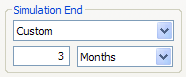
   This setup runs the simulation for three months. Run Setup can also control when simulation starts, where to write report results, and other general simulation setup information.
   
   
3. Click the Cancel button, since we are not changing simulation setup.

What-If Analysis and Simulation

You can use the power of discrete event simulation and analysis to improve your processes. 

Example

You are a manager whose goal is to increase throughput by reducing average lead time through the process. Currently, it is taking too long to ship an order, orders are stacking up unfulfilled, and your competitors are about 10-20% faster. You'd like about a 25-30% increase in production, and corresponding reduction in time to ship an order, to clearly differentiate yourself from your competitors.

Topic Tasks

Start the Simulation
Use the Report Window
What-If Analysis #1: Add Parallel Processing
Results of the First What-If Simulation (The Report Window)
Change Tables to Report Graphs
What-If Simulation Analysis #3: Resource Utilization and Constraints
Results of the Third What-If Simulation (Report Window) 

Start the Simulation

Click the Start button 

 on the Modeling toolbar.
A full three months of process time is simulated in seconds, and a Report window appears. 

Use the Report Window

iGrafx provides simulation report statistics categorized by tab: Time, Cost, Resource, Queue, and a Custom tab where you can collect key statistics that are of most interest. On the Custom tab, you can copy and paste report elements from other tabs or, on the Report menu, choose Add Element to create the Custom tab content. 

1. Click each of the Report tabs to view the various statistics gathered. Statistics are shown that help you understand the time to perform the process, the costs involved, the resources utilized, and the queueing (lines or bottlenecks) that develops.
2. Click the Custom tab.

The first statistic you'll analyze is cycle time, also known as lead time. Cycle time and the count of Orders Shipped are shown in the first table of the Custom tab. 
The Production organization (represented by the Production swimlane) claims that if they received orders sooner, cycle time could be reduced. Before changing the business, you test the idea with iGrafx. 

What-If Analysis #1: Add Parallel Processing

Production can work on an order at the same time as the credit organization (a parallel path). If the order is stopped due to bad credit, we will use a Discard command to cancel the order in both organizations.

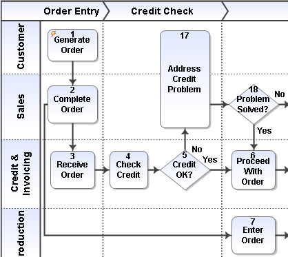
1. From the Window menu, choose the Order Fulfillment process.
   
   You can also double-click the Order Fulfillment process in the Explorer bar to view it. 
   
   
2. Click the line between Proceed With Order (shape 6) and Enter Order (shape 7) and press the Delete key.
3. Draw a line from Complete Order (Shape 2) to Enter Order (Shape 7).
   See Connect Shapes in this tutorial if you need a reminder about how to draw a line.
   
   A portion of your diagram may now look like this: 

Set the Stop Order shape to discard the transaction in production:

If there is some problem with the Credit Check that we cannot address with the customer, we must stop the order. This means telling the parallel production path to stop all work on this order. We will use the Discard functionality to tell Production to stop work:

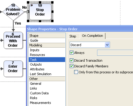
1. Double-click the Stop Order shape.
2. Select the Task page.
3. Click the On Completion tab.
4. Choose Discard from the drop-down list.
5. Select the Discard Family Members check box. Your dialog should now look like the picture below:
   
   

   

    
   
   
6. Click OK to save your changes.

In our modified process, orders duplicate at the Complete Order activity to allow parallel work on an order by two organizations. When transactions duplicate in iGrafx, they are considered part of the same family, like twins. The Discard Transaction setting cancels the transaction in the Sales organization. The Discard Family Members setting cancels the parallel transaction in the Production organization. 

Append additional simulation statistics to the existing report:

1. Click the Run Setup button 

   

    on the Modeling toolbar.
2. Click the Initialization/Reports tab.
3. Click the Append to Report option.
   
   

   

    
   
   
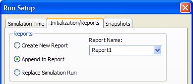
4. Click OK.
5. Click the Start button 

   

    to run the simulation again.

Results of the First What-If Simulation (The Report Window)

When the simulation is complete, the Report window appears, and the statistics from the latest simulation are appended to the earlier results because we set up the simulation to Append to Report.

Click the Custom tab, if it is not already shown, and review the statistics for Shipped Orders. 

The process cycle time and throughput count has not changed significantly, so the idea from Production won't help much. We should continue our analysis. An employee tells management, "You know, we check the customer's credit on every order, and that keeps the Credit & Invoicing organization very busy. What if we only checked the credit of new clients?"

This is the idea we will test next. However, we first want to name our simulations. 

Name the latest simulation:

This indicates what improvements were made and gives a more descriptive name to the headings in report elements.

1. Ensure the Report window is shown.
   
   From the Window menu, choose Report1 if it is not displayed. You can also choose Report1 in the Document Components window.
   
   
2. From the Report menu, choose Simulation Data.
3. Under Simulation Names, double-click Sim #2 (or click on it and then click the Name button).
4. Type a new name, such as "Parallel Production".
5. Click OK, to save changes and close the Name Simulation Data dialog box.
6. Click the Close button in the Simulation Data dialog box.

All of the headings in the report elements now reflect the new name. 

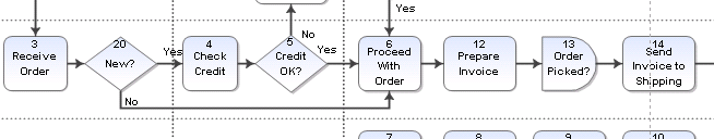
What-If Simulation Analysis #2: Improve the Credit Check

We will now change the process to check credit only on orders from new customers.

1. From the Window menu, choose the Order Fulfillment process.
2. Click the Order Entry phase header at the top of the diagram, then place your cursor over the dark square at the right edge of the phase.
3. Click and drag the dark square to near the right edge of the text in the Credit Check phase to extend the phase.
4. Place a Decision diamond on the line between Receive Order (shape 3) and Check Credit (shape 4). For a reminder about how to place a decision shape, see Place Decision Shapes.
5. Type "New?" to label the decision.
6. Right-click over the "No" decision line and choose "Yes" to switch the paths.
7. Draw a line from the New? decision shape to Proceed With Order (shape 6). For a reminder on how to draw lines, see Connect Shapes.
8. Double-click the New? decision shape.
9. In the Properties dialog box, click the Guide page.
   
   The default percentage for a decision is 50% yes or no. Assume that only 50% of the new orders come from new customers. You can always change this later for more what-if analysis.
   
   
10. Click OK.
    
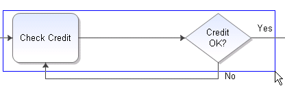
    The changed portion of your diagram may look like this: 
    
    

    

     
    
    
11. Click the Start button 

    

     to begin the simulation.

Results of the Second What-If Simulation (Report Window)

The Report window is visible again after running a complete simulation. 

1. Click the Custom tab of the Report window, if it is not already shown. Note that a simple change to the process has resulted in decreased cycle time and improved throughput!
2. Name the simulation; for example, "Less Credit Check". (For a quick reminder, see Name the latest simulation.

Change Tables to Report Graphs

You can show any of the report elements in the simulation report as a table (the default) or a graph.

1. Double-click the Orders Shipped (Days) report element at the top of the Custom report.
2. Click the Format tab and change the Display As setting to Graph.
3. Click the Graph Style button.
4. Click the Line graph button.
5. Click OK to save changes and close the Graph Control dialog box.
6. Click OK to save and close the Edit Report Element dialog box.
   
   Your report element is changed to a line graph.

Make a copy to show the data in table format:

1. Select the report element (the line graph you created) by clicking on it.
2. Press and hold the Ctrl key while you press the C key (Ctrl+C) to copy the Report Element or, on the Edit menu, choose Copy.
3. Press Ctrl+V to paste the element or, on the Edit menu, choose Paste.
4. Double-click the bottom graph.
5. Click the Format tab and change Display As to Tabular.
6. Click OK.

What-If Simulation Analysis #3: Resource Utilization and Constraints

Next you'll review the utilization of resources, where constraints on order flow (bottlenecks) are occurring, and do some what-if analysis with your resource allocations. 

Scroll down in the Custom tab of the report until you reach the Resource Utilization graph and table. 

Giving Credit & Invoicing less work reduced their utilization, and yet you still have organizations that are very highly utilized. 

Scroll down to the Average Waiting Time for Transactions that Waited graph. How long did orders wait for each organization? 

The Production organization is, by far, the most significant bottleneck. You can hire someone in Production and see if it helps throughput. 

1. Click the Resources button 

   

    on the Modeling toolbar.
2. In the Define Resources dialog box, expand the Person folder and click Production.
3. On the Properties tab, change the Resource Use from Individual to Pool and the Count to 2.
4. Click OK.
   
   This information is part of a Scenario, the environment where the process is simulated. To view the Scenario window, from the File menu, choose Components to view the Document Components window, then double-click on the Scenario you want to view. In the Document Components window, you can right-click a Scenario to create a new Scenario, or copy and paste Scenarios. If you view the Scenario, click the X button in the upper-right corner of the window to close it 
   before you do the next step.
   
   

5. Click the Start button 

   

    to simulate.

Results of the Third What-If Simulation (Report Window)

The performance improves, but the bottleneck has moved! The Shipping organization now receives all the work that the Production organization was holding up. You have optimized only a portion of the process, and not the overall process. This is a good example of how iGrafx can show the unexpected consequences of changing a process or staffing levels.

Name the latest simulation (Sim #4) "Hire Production". For a quick reminder, see Name the latest simulation.

Six Sigma Analysis: Interface with a Statistical Application

iGrafx Process for Six Sigma provides powerful functionality for Six Sigma, including integration with the leading statistical packages MINITAB® & SAS JMP®. If you have the iGrafx Process for Six Sigma client software, you can perform full Design Of Experiments (DOE) analysis, logging statistics for every transaction to the statistical application, and even perform path- walking analysis. 

Topic Tasks

Use Fit Data to Refine the Simulation Model
Using RapiDOE to Perform a Design Of Experiments

Use Fit Data to Refine the Simulation Model

Up to this point, this tutorial has used Subject Matter Expert (SME) guesses or anecdotal data to guide our simulation analysis. While this data can be accurate enough to perform powerful simulation analysis, you can refine your simulation model further with empirically measured data from the actual process. 

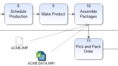
The time for the Assemble Packages step in the Production organization is one of the longest in the ACME Order Fulfillment Process (ACME_Order.igx in your Sample directory). Maybe the time based on the SME opinion is not as accurate as possible. After a study of 30 different orders at the Assemble Packages step, we have captured those times in the statistical package. 

Open the statistical package on captured data:

MINITAB or JMP must be installed on your machine for this feature.

1. Ensure the Process diagram is shown.
   
   From the Window menu, choose the Order Fulfillment process. 
   
   

2. Double-click the MINITAB or JMP icon near the Assemble Packages step, based on which application you have loaded on your machine.

   

   The following pictures and instructions assume you have chosen MINITAB. In general, the instructions also work for JMP

   
   

   

   
   
   

3. After the statistical package starts, click the iGrafx Process for Six Sigma icon in the Windows task bar to return to it.

Perform a statistical curve fit on the empirically measured data captured in the statistical application:

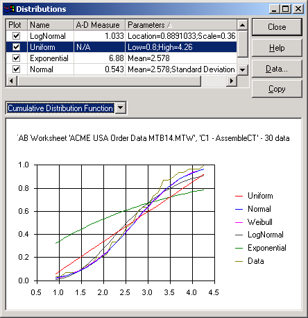
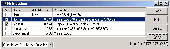
1. From the Six Sigma menu, choose Fit Data. The Distributions dialog box and the Choose Data dialog box appear.
2. Ensure that the AssembleCT column is chosen in the Choose Data dialog box, and click OK.
   iGrafx uses the statistical package to perform analysis, and then graphs the resulting analysis for you.
   
   

   

    
   
   You can click and drag a corner of this dialog box to make it bigger. 
   
   Some distributions are a better fit than others. Look for the closest fit to the actual data (and, if using MINITAB, for the lowest A-D Measure). You can see that the Exponential, Uniform, and LogNormal functions don't fit very well, so we will remove them from the plot. 

Remove functions from the plot:

1. Clear the Exponential check box in the plot column, and notice it is removed from the plot.
2. Clear the check boxes for Uniform and LogNormal.
   
   Normal and Weibull both seem to fit the data very well.

Choose the Normal data distribution:

The Central Limit Theorem says data tends towards normality, and Weibull is capable of adjusting itself to match Normal curves, so we should choose the Normal distribution.

1. Click the Normal line in the table to select it.
2. Click the Copy button to copy the Normal Distribution shown below the button.
   
   

   

    
   
   
3. Click the Close button to close the Distributions dialog box.

Adjust the properties of the Assemble Packages activity with empirically measured data:

1. Double-click Assemble Packages (shape 10) to display its Properties.
2. Click the Guide page.
3. From the Time drop-down list, choose Expression.
4. Select (highlight) the text for the current expression ("Between(2,4)").
5. Right-click in the expression window and choose Paste (near the bottom of the context menu).
6. Click OK.

You have refined your simulation model with empirically measured data. You could now run simulation analysis on single factors. However, a a Design of Experiments or DOE analysis would be more comprehensive and powerful. 

Using RapiDOE to Perform a Design Of Experiments

This section of the Tutorial assumes that you have either been trained on Design of Experiments (DOE), or have a basic understanding of the purpose (and limitations) of doing a DOE. MINITAB or JMP must be installed on your machine for the RapiDOE feature. 

The One Factor at A Time (OFAT) simulation analysis you did so far may miss interactions between the factors you have been changing. Instead of changing the resources one at a time by hand, you can perform a DOE analysis on the process and try many different combinations of resource levels automatically. With DOE, you can change several factors at once and easily analyze the results in iGrafx or in the statistical package. 

Use the RapiDOE functionality in Process for Six Sigma:

1. From the Six Sigma menu, choose RapiDOE.
   
   The RepiDOE dialog box appears, shown here with relevant sections on Available Factors and Responses expanded:
   
   

   

   
   
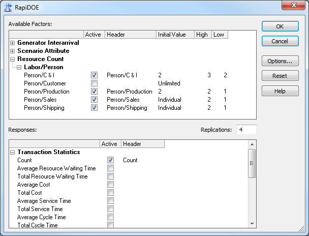
   The RapiDOE dialog box displays the Factors and Responses that you can choose for a DOE on a simulation model. Factors can include Generator behavior, Scenario Attributes, and Resource Counts. 
   
   In this RapiDOE topic, we have setup the DOE to add one person to the original resource level in each organization. Responses can include transaction statistics such as cycle time or count completed, Scenario Attributes, or Custom Statistics that you define. This topic guides you to track Transaction (order) Completion Count and resource costs, and look for the total number of orders produced and the resource cost involved in producing the orders. 
   
   Although you can use the Options button fractionalize the design or choose a general factorial experiment with a center point, fractionalizing the design makes results less accurate. Running additional simulations on our model with iGrafx is fast. 
   
   Use the Replications number to control how many times each experiment is replicated, to introduce more randomness into the DOE. Choose replications cautiously; replicates help make results more accurate, and they also multiply the number of simulations to run.
   
   
2. Click OK.
   
   The Run Experiment dialog box appears.
   
   This DOE defines 64 different simulations to run: 2-level full-factorial design on 4 factors is 24, or 16, times 4 replicates each, for a total of 64.
   
   
3. Click Start to run the 64 different simulations.
4. When simulation completes, iGrafx will indicate the data has been stored to the statistical application (e.g. a MINITAB Worksheet Name is given when using Minitab). Note the name of the sheet, and OK the dialog box.

Sort results within iGrafx:

We will now sort responses so you can see if there is a pattern of factors that have an impact on the responses. This is sometimes known as "Analysis of Good," or ANOG. You may need to make the dialog box bigger to see all columns of data.

1. Click once on the Count column to sort in ascending order.
2. Click again on the Count column to sort in descending order.
   
   The highest number of orders (transactions) is produced when Production and Shipping both have 2 people working. The Sales organization varies between 1 and 2, and Credit & Invoicing varies between 2 and 3. Production and Shipping are solidly at 2 for the higher transaction counts. 
   
   The ANOG suggests that if we ensure you have two people each in Production and Shipping, you should be able to reach around 80 or more orders per quarter. 
   
   
3. Click Close to close the Run Experiment dialog box.

Use the simulation to confirm the results of the DOE:

We will now add a resource to the Shipping organization to test our theory that we can increase throughput with one additional hire. You already added a resource to Production in previous experiments. 

1. Click the Resources button 

   

    on the Modeling toolbar.
2. In the Define Resources dialog box, expand Person, and click Shipping.
3. On the Properties tab, change the Use setting from Individual to Pool and the Count to 2.
4. Make sure the number of Production persons also has a Pool count of 2.
5. Click OK.
6. Click the Start button 

   

    on the Modeling toolbar to simulate.

Results of Confirming the DOE (Report Window)

The bottleneck has been apparently been removed; resource utilization has gone down, and (more importantly for determining bottlenecks) the Average Waiting Time has also been significantly reduced in all organizations. 

1. Scroll up to the top of the Custom tab of the report, and review overall production in the top report element graph and table.
   
   Cycle time is dramatically reduced, and throughput is significantly increased! Resource constraints and other sources of bottlenecks can have a dramatic and hard-to-predict impact on a process. 
   
   With simulation, you can build a business case for change, with statistics to back up your proposals, all without impacting the actual production process or incurring excessive costs. 
   
   
2. If you are familiar with DOE analysis in MINITAB or JMP, you can now move to that application and perform further analysis if you want to.
3. Close the ACME_Order.igx file, saving your work if you want to. If you want to save changes, on the File menu, choose Save As and give the file a new name.

Cause and Effect Diagrams

Cause and Effect (CE) diagrams are sometimes referred to as Fishbone or Ishikawa diagrams. The CE diagram methodology represents the relationships between an effect and all possible causes influencing it.

Topic Tasks

Create a New CE Diagram
Edit the Default Effect
Edit Causes and Sub Causes
Insert Causes
Adjust Layout
Update the Error Column
Export a CE Diagram to an FMEA

Create a New CE Diagram

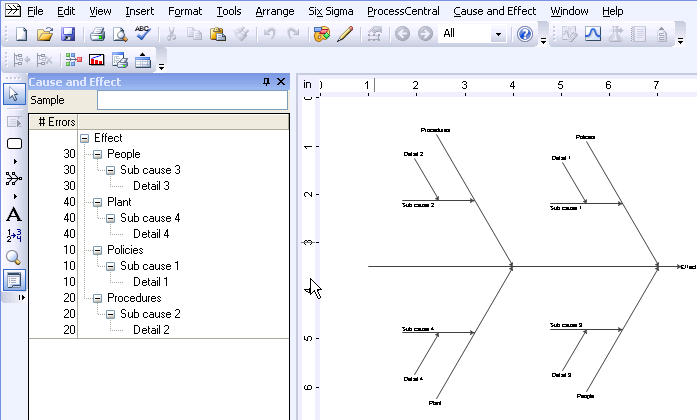
From the File menu, select New, and in the resulting New dialog box, choose the Cause & Effect template category, then choose Cause and Effect (Transactional) and click OK.

A new CE diagram opens, with default values that are ready to edit.

 

Edit the Default Effect

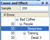
When you change the main effect in the Cause and Effect window, it automatically updates the CE diagram.

1. Click the Effect text in the Cause and Effect window.
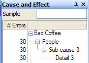
2. Type in a new Effect. For example, type in Bad Coffee. Your Explorer bar may look like this:
   
   

   

    
   
   
3. Press the Enter key to save your changes to the Effect.
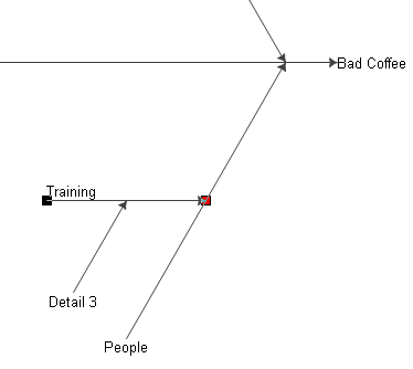
4. The main effect arrow updates automatically to show the new main effect.

Edit Causes and Sub Causes

After you have documented the effect, you can detail its primary causes, such as People, and subcauses. (Subcauses are causes of primary causes.) 

1. Click Sub cause 3, under the People cause in the Cause and Effect window, and type "Training" for the new value.
   
   

   

    
   
   
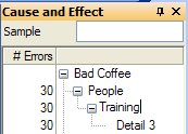
2. Press the Enter key when finished.
3. The CE diagram automatically updates to show the new value: 
   
   

   

    

Insert Causes

You probably have more than one subcause for any given primary cause for the effect.

1. In the Cause and Effect window, right-click the People cause and choose Add Cause:
   

   

    
   
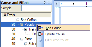
   The new cause is inserted at the end of the subcause list for the cause that you right-clicked.
   
   
2. Type "Sleepiness" for the new subcause.
   

   

    
   
   
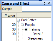
3. Press the Enter key to finish your edits.

Adjust Layout

If you want to change the look of the current CE diagram, you can change the layout options to redraw it. Note that if you do this, you will lose any manual layout changes you have made.

1. Right-click in the Cause and Effect window and choose Layout Options.
2. Use the controls in the Layout Options dialog box to modify different aspects of the diagram. For example, you could rotate text to be the same direction as the CE line (branch) they are on.
3. Click Apply to try out a layout, or simply click the OK button.
   
   The CE diagram is updated with your new layout. 

Update the Error Column

This procedure updates the number of errors for a subcause you've added. Errors appear in the Errors column of the Cause and Effect window. Updates in the Cause and Effect window also appear in the CE diagram.

1. Click the Error column next to the Sleepiness subcause.
2. Type "50" for the number of errors observed, then press the Enter key.
3. In the Sample text box, enter "200" for the total number of samples.
   
   

   

    
   
   
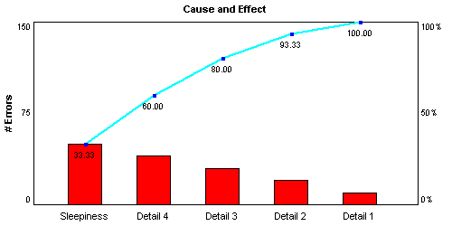
4. Insert a Pareto Chart based on the number of Errors. To do so, on the Cause and Effect menu, choose Insert Pareto Chart.
5. Scroll down the diagram to view the Pareto chart.
   The Pareto chart will automatically update to show the new data:
   
   

   

    

Export a CE Diagram to an FMEA

The information from a CE diagram is often an excellent starting point for doing a Failure Modes and Effects Analysis (FMEA).

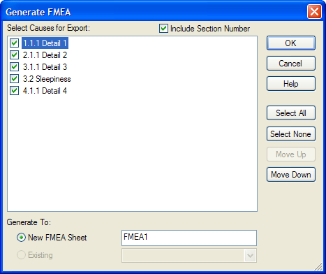
1. From the Cause and Effect menu, choose Export to FMEA Sheet.
   
   The Generate FMEA dialog appears:
   
   

   

    
   
   
2. Select which of the listed causes you want to export; by default, all causes are selected.
3. Enter the name of the new FMEA and click OK.
   
   If you had previously exported to FMEA, the Existing option would also be available.
   
   
4. Confirm the name of the New Component and click OK.
   
   The FMEA Sheet appears. You can now fill in the sheet, including Severity and Detection numbers. (Occurrence is filled in from the Error column using the Sample size you entered.) Once you have entered Severity, Occurrence, and Detection numbers, the Risk Priority Number (RPN) is calculated, allowing you to rank the various causes and sub-causes in order of importance. To learn more about FMEA, read the iGrafx Help. 

BPMN Diagrams

BPMN diagrams and data have unique terminology. This tutorial assumes that you are familiar with BPMN terms. You may find it helpful to review the iGrafx Help system documentation on BPMN terminology. Another source for BPMN information is http://www.bpmn.org/.

Topic Tasks

Creating a BPMN Diagram
Place Shapes (BPMN Flow)
Set Shape Behavior
Place, Connect, and Set Shape Behavior
Check a BPMN Diagram

Creating a BPMN Diagram

From the File menu, select New, choose the BPMN category, and then choose BPMN Basic Collaboration.
A sample BPMN diagram opens. 

Place Shapes (BPMN Flow)

For a reminder of how to place shapes, see Place Shapes (Activities) at the beginning of this tutorial.

1. Click on the activity shape 

   

    on the Toolbox toolbar.
2. Move the cursor into the diagram, and put it over the circular Event shape on the left side of the diagram.
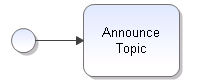
3. Click and drag the outline of the new shape to place it at the right of the Start shape
4. Now label the shape "Announce Topic." Your map may look like this:
   
   

   

    
   
   
5. Add an event shape and another activity, then enter text in the shapes so your diagram looks like this:
   
   

   

    
   
   
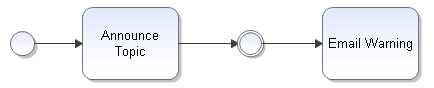
6. Note that the event is automatically formatted to be the correct dimensions (e.g. an intermediate event) based on which lines you have drawn. iGrafx intelligently adjusts BPMN diagram shapes based on the requirements in the BPMN specification. 

Set Shape Behavior

Change the intermediate event type to a delay:

1. Double-click the intermediate event, the one after the Announce Topic shape.
2. In the Properties dialog box, select the BPMN Guide page and set it to a Delay Timer as shown below:
   
   

   

    
   
   
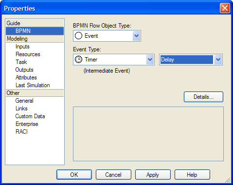
3. Click OK.
   
   The graphical symbol for the event is now updated to reflect the behavior you have specified:
   
   

   

    

Place, Connect, and Set Shape Behavior

Next, you will add, connect, label, and change activities to match proper BPMN behavior. 

Place, connect, and label some new shapes:

Place two more shapes as shown below: 

 

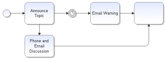
For a reminder of how to place shapes, see Place Shapes (Activities) at the beginning of this tutorial. 

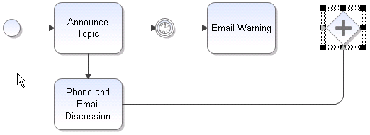
Change the behavior of the unlabeled shape to properly synchronize the parallel paths:

1. Double-click the unlabeled activity at the right of the diagram.
2. In the Properties dialog box, select the BPMN Guide page and change the Activity to a Parallel Gateway, as shown below:
   
   

   

    
   |
3. Click OK.
   
   Your diagram is updated with the new type of BPMN object you specified: 
   
   

4. 

    

Check a BPMN Diagram

The BPMN diagram type contains dynamic real-time checks to help you draw a correct-by- construction diagram that complies with the BPMN specification. 

Try correct-by-construction design features:

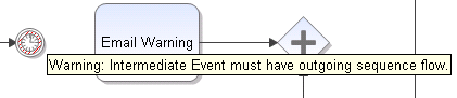
1. Delete the line between the Timer event and Email Warning. The Timer indicates a design problem with shaded red lines.
2. Place your cursor over the shaded Timer event. A yellow tooltip describes the problem:
   

   

    
   
   
3. Press Ctrl+Z on your keyboard to restore the line (undo) or, from the Edit menu, choose Undo Clear.
   
   We recommend that you leave real-time checking on, even though you can turn it off on the View menu. 
   
   In some cases, it is not possible or desirable to enforce correct-by-construction modeling. For these situations, BPMN diagrams have extensive static checking features. 

Perform a static check on this diagram:

1. From the Model menu, choose Check. The Check dialog box appears:
   
   

   

   
   
   
   

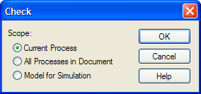
   You may perform a check on this diagram, on all diagrams in this document, or perform a check to ensure this model is ready for simulation with iGrafx clients that allow simulation

2. Click OK to check this diagram. A warning appears in the output window at the bottom of the screen:
3. Gateway must be followed by an End Event.
   
   "Containing process must use Start/ End Events consistently."
   
   
4. Double-click the warning message to highlight the source of the warning in the diagram.
   
   In this case, if you place and route an Event type flow object to the right of the gateway, at the end of the sequence flow, it will solve the problem. You can verify this by re-checking the diagram. 

Organization Charts

You can quickly create high-quality organizational charts with iGrafx.

Create a New Organization Chart

From the File menu, select New. In the resulting New dialog box, choose the Business category, then choose OrgChart and click OK.

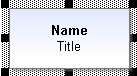
A single shape that represents a role in the organization is the starting point for your chart:

 

The OrgChart Builder and OrgChart Data Editor dialog boxes help you rapidly create and modify organization charts: 

 

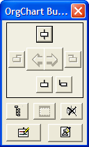
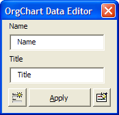
If these dialog boxes are hidden, you can access them from the OrgChart menu. 
Most OrgChart Builder commands require you to select a role (shape) before using the command. 

Set Name and Title

1. Select the shape, then enter the Name and Title text you want in the OrgChart Data Editor.
   
   

   

    
   
   
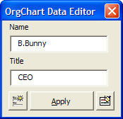
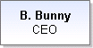
2. Click the Apply button.
   
   The shape updates with the data you entered: 

 

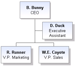
Add Subordinates

1. Select the B.Bunny role.
2. In the OrgChart Builder dialog box, click the Add Subordinate tool: 

   

3. Add subordinate shapes and give them the names and titles R. Runner, V.P. Marketing and W.E. Coyote, V.P. Sales. 

Add Assistants

1. Select the B.Bunny role.
2. In the OrgChart Builder dialog box, click the Add Assistant tool: 

   

3. Name the Assistant D. Duck, and type the role Executive Assistant Your diagram may look like this:

 

Add Co-Workers

1. Select W.E. Coyote role.
2. In the OrgChart Builder dialog box, click the add co-worker to the right tool: 

   

    
   
   The OrgChart updates with the new co-worker shape:

 

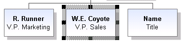
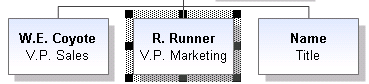
Re-Order People Within the Team

1. Select the R. Runner role.
2. In the OrgChart Builder, click the right-arrow button 

   

    .
   
   The OrgChart updates with the new position of the role:

 

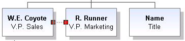
Show Dotted-Line Relationships

1. Place your selector tool cursor inside the W.E. Coyote role.
2. Click and drag to the left side of the R. Runner shape. Your chart now shows this dotted-line relationship:

 

Change Workgroup Layout

You may set or change the layout style of roles in your workgroup in relation to each other.

1. Select the B. Bunny role.
2. In the OrgChart Builder dialog box, click the Workgroup Layout Styles tool: 

   

   
   
   The Workgroup Layout Styles dialog box appears:
   
   

   

    
   
   
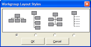
3. Click a different layout style option, then click OK to apply the style.

Your selection sets the style for the subordinates and assistants you have not yet added. 

Congratulations! You have reached the end of the tutorial.